
Understanding FSR 4
AMD accidentally leaked the FSR source code, let's see how it works!


FidelityFX Super Resolution (FSR) is AMD’s line of real-time image upscalers that compete with Nvidia’s Deep Learning Super Sampling (DLSS) technology. The goal of these technologies is to allow game developers to render at a lower resolution (with high performance) and then upscale the image into a higher-resolution more detailed version. Since these technologies have to run in real-time in the “left over” time after a frame is generated, they have to be quite performant, typically taking less than 1ms to go from say 720p render resolution to 1440p display resolution. FSR has traditionally been seen as lagging behind DLSS, but it was open source and cross platform (working on all GPUs). DLSS leveraged Nvidia’s lead in deep learning technology while FSR relied on more traditional heuristic methods. The situation changed with the release of FSR 4. Unlike previous iterations, this time AMD was advertising a new deep-learning based system. Reviews were very positive, indicating that AMD has nearly caught up to Nvidia in this space. Unfortunately, unlike previous iterations of FSR, FSR 4 was closed source and restricted to GPUs with AMD’s latest RDNA 4 architecture.
Then, in August AMD engineers accidentally uploaded the FSR 4 source code to the to the official FidelityFX github page. Gamers were excited to find an unreleased implementation of FSR 4 for older GPUs (based around int8 instead of fp8 arithmetic) that was quickly compiled into a DLL that could be swapped into their GPU driver. I was excited to find out how the technology worked. After looking around online to find an analysis and coming up short, I decided to read the code myself.
The DLSS and FSR 4 technologies are pretty impressive. Research implementation of super resolution networks can take several seconds to produce a single HD-resolution frame. These technologies are 1000x faster than that. Based on those research papers I expected to find a U-Net architecture that took low resolution RGB pixels as input (perhaps from a series of previous frames) and output high resolution RGB pixels. I was surprised to instead find that FSR 4 is really an evolution of the FSR 2 technology with some of its simple heuristics replaced by a neural net. Therefore in order to understand how FSR 4 works we must first briefly cover FSR 2.1
FSR 2
Since FSR 2 is part of AMD’s GPUOpen, it’s quite well documented. I found this video helpful in understanding how it works:
At its core FSR 2 works by sampling different sets of pixel in different frames and then accumulating that information over time. This puts it in the general class of algorithms known as Temporal Anti-Aliasing (TAA)2. A good overview of TAA techniques can be found here but I’ll give a brief summary. Figure 1 shows how a static scene that contains a high resolution square pattern in the center would be rendered in a TAA implementation.
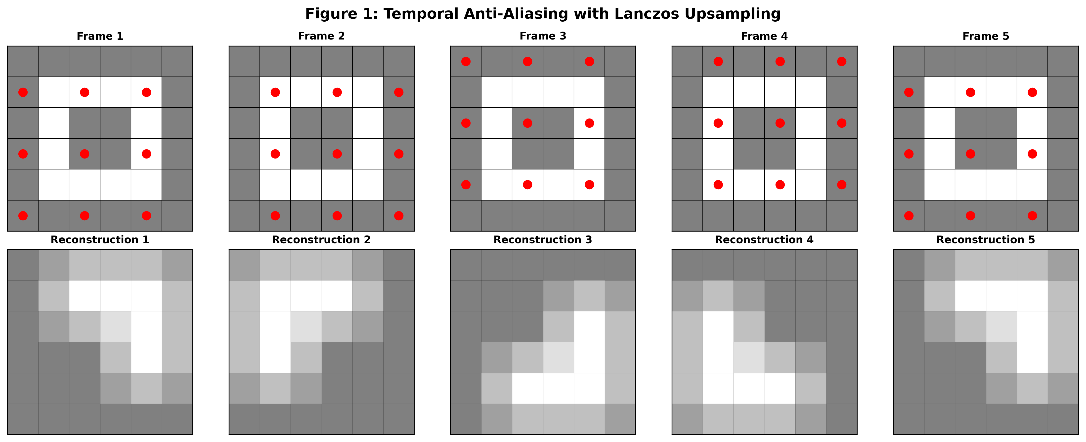
In this figure a static scene is rendered across five frames. The red dots on the top row represent the sampled points in each frame. In the bottom row are the resulting upscaled reconstructions from the sampled points for each frame. This low resolution sampling is insufficient to accurately reconstruct the scene on a frame-by-frame basis. Note that for simplicity above we are showing a well-ordered sequence of points that will cover the whole space of output pixels in four frames. The real FSR uses a Halton sequence to pseudo-randomly cover the space eventually.
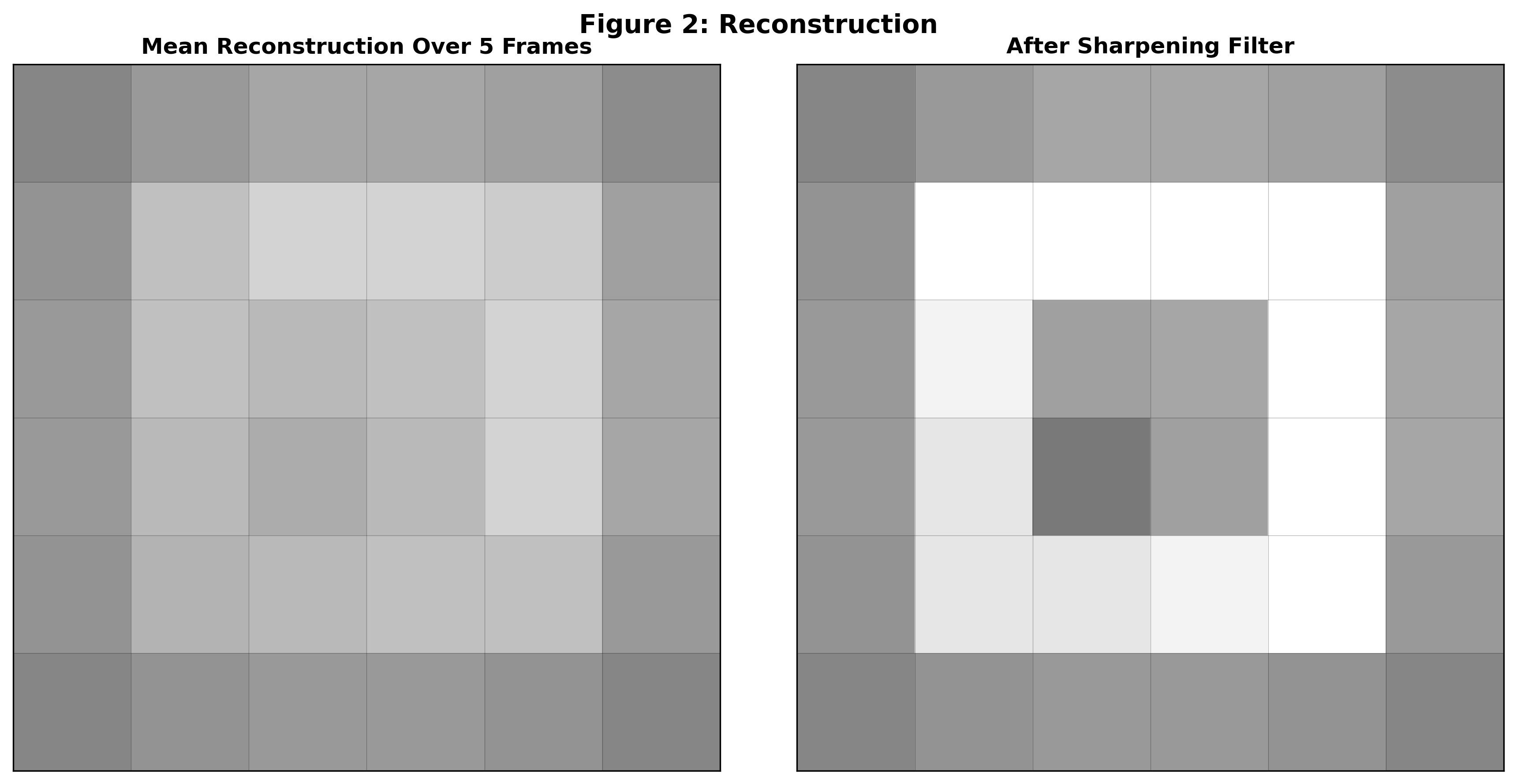
If we average across frames we get a blurry image that contains high-resolution information that wasn’t available in the individual sample frames. In order to get a non-blurry image we can apply a sharpening filter. AMD has developed a sharpening filter called Contrast Adaptive Sharpening (CAS) that tries its best to mitigate issues that can arise with naive sharpening filters.
TAA works great with static scenes, but there are issues when objects are in motion. If no motion correction is performed then averaging frames over time will cause motion blur. In order to get around this, FSR (like other TAA implementations) asks game developers for motion vectors that describe for each output pixel in the current frame where the corresponding object pixel was in the previous frame. That lets FSR reproject the previous frame’s pixels into their current locations and therefore allow it to build up a high resolution image even in the presence of movement.
This works well in the middle of a moving object but can cause artifacts in the edges since the motion vectors are usually provided in low-resolution form. Problems also often arise with particle effects or other times when the color of an object changes rapidly but the game engine cannot provide motion vectors that point to similar pixels from the previous frames. Another difficult challenge in TAA is disocclusion. This is when a foreground object moves and reveals objects in the background. In these cases FSR has no historical data from previous frames to work with and must produce the upscaled image from scratch.
In order to handle edges, particle effects, and disocclusions, FSR 2 has an array of heuristics that decide when to sample information from further in space (causing a more blurry image) or further in time (risking motion blur). These heuristics sometimes fail and cause artifacts like smeary motion or shimmering edges which is why FSR 2 was seen as an inferior system to Nvidia’s DLSS. More details of these heuristic techniques and the associated artifacts can be seen in the TAA explainer linked above. It looks like AMD’s engineers realized that replacing hand-tuned heuristics is one of the best applications of machine learning and therefore leveraged the neural network specifically for this task.
FSR 4
FSR 4 consists of three steps: a feature engineering step, the neural network, and a filtering/upscaling step. It will make more sense to work backwards.
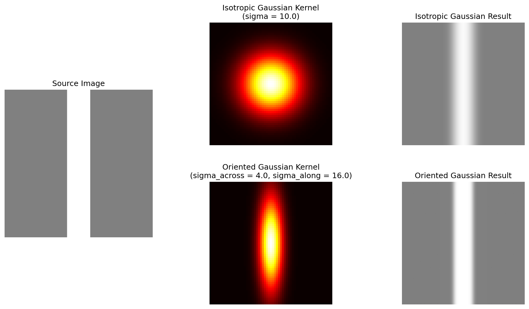
The upscaling stage of FSR 4 works very similarly to the upscaling and temporal averaging process of FSR 2 described above. However instead of a symmetric spatial filtering kernel, FSR 4 uses oriented Gaussians whose parameters are specified by the neural network for each output pixel. If the Gaussian is correctly oriented, this can dramatically increase the sharpness and perceived resolution of the output. To understand why, consider a bar being upscaled by FSR 4. If the output is constructed using a round filter, the bar gets smeared but with an oriented Gaussian the effect is much less pronounced.
The network also outputs a blending factor which determines how much influence past frames should have on the current frame. If the network determines that the scene is changing rapidly in ways that cannot be compensated for by motion vectors (for instance due to particle effects or disocclusion) it will reduce the influence of past frames and it will instead rely on a best-effort reconstruction using the oriented Gaussians in the spatial filter. The method of predicting filtering kernels instead of directly predicting the output pixels is known as a Kernel Prediction Network and was originally developed for image denoising.
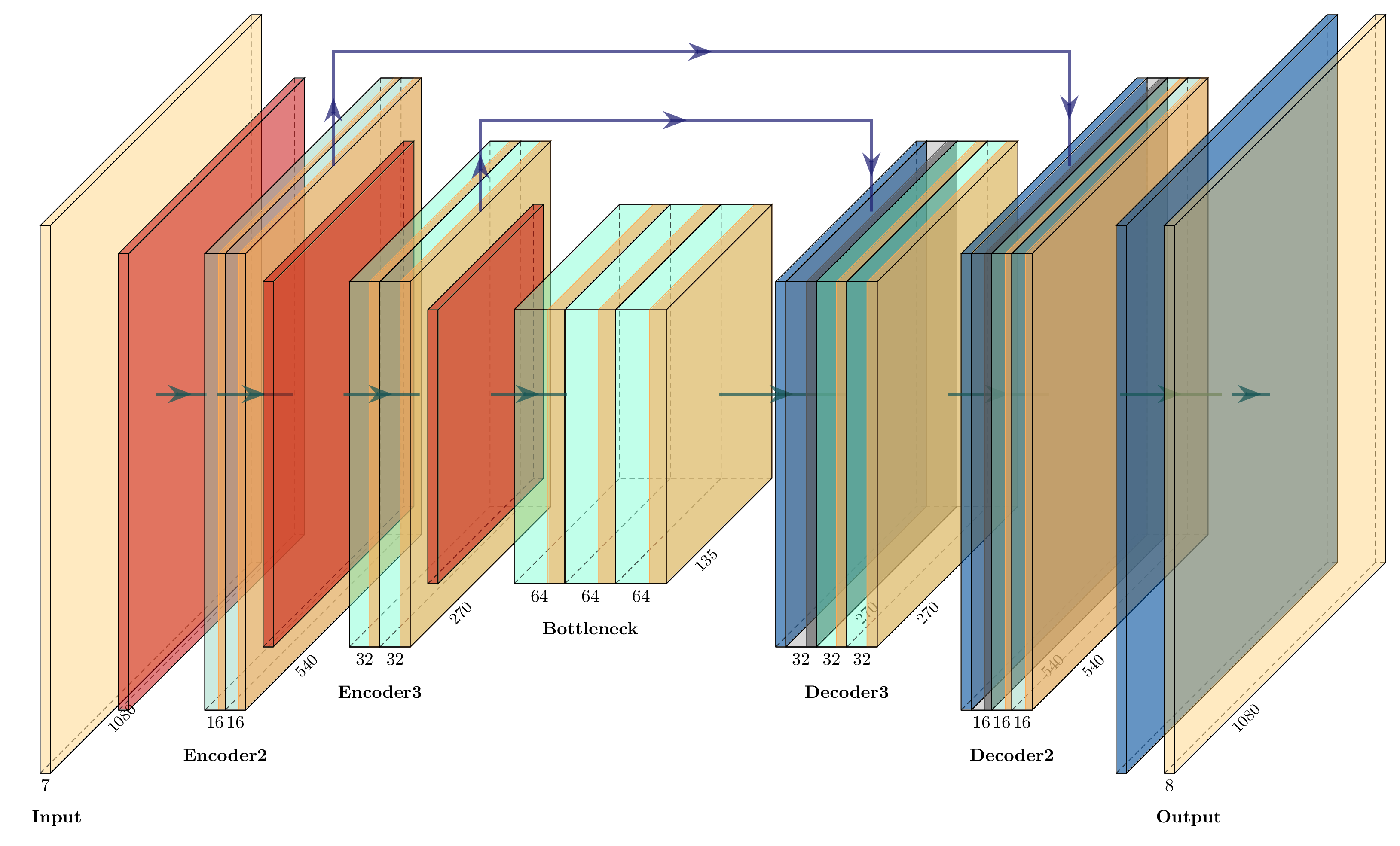
The neural network takes 7 values as input and produces 8 values as output for each output pixel. Three values are used to produce the oriented Gaussian (height, width, and tilt3) and one value is used as the temporal blending factor. The remaining four values are recurrently passed back into the network in the next frame. That way the network is able to “remember” important information over many frames. The inputs to the network are those same four values from the previous frame as well as a grayscale representation of the current frame (naively upscaled to the target resolution), a grayscale version of the previous output frame, and a value that represents how colorful that pixel is. The network therefore runs at the output resolution. In order to fit into the 1ms budget, this network has to be tiny by modern deep learning standards. It’s a 39-layer U-Net architecture with 3x3 spatial convolution extents and aggressive strides/downsampling. It has only around 100k parameters, making it 10x smaller than even early neural networks targeting mobile devices. The network is compiled from an ONNX representation into HLSL by AMD’s ML2Code. Interestingly, AMD engineers took the generated code and manually “kernel fused” the preprocessing step into the layer 1 ML kernel and the filtering step into the layer 14 ML kernel in order to get some extra performance. I’ve created a more detailed breakdown of the network at the bottom of this post.
The feature engineering step of FSR 4 is in some ways pretty simple. Like FSR 2 it uses upscaled motion vectors to reproject the previous frame into the current frame’s locations. A depth map is used to do this more accurately (similar to how it’s used for FSR 2). But the feature engineering step has one more clever trick up its sleeve: it also reprojects the four per-pixel recurrent neural network states using the motion vectors. This means that rather than forcing the network to learn motion compensation internally (as most temporal neural networks do), FSR 4 explicitly warps the recurrent memory to follow moving objects. This “free lunch” from the game engine’s motion vectors simplifies what the network needs to learn, allowing AMD to achieve high quality with an extremely compact model. To my knowledge this technique of reprojecting the recurrent signals of a neural network has not been previous published.
Conclusions
Richard Sutton’s bitter lesson says that techniques that can leverage the enormous amount of compute generated by Moore’s law will eventually beat out techniques that directly encode human knowledge and engineering. However, in the field of real-time graphics, compute is still very constrained. That means there is still an important place for feature engineering. It was fun for me to deconstruct the thoughtful work AMD engineers have put into this product. The details of the implementation also shed light on why FSR 4 and DLSS struggle in certain scenes like those with particle effects and when content is shown on an in-game screen. Under these conditions the algorithms do not have motion vectors to tell them where to sample from previous frames and the result is heavy motion blur. As AMD and Nvidia work to address these problems in future updates, I hope they will release more information about their algorithms so we can all benefit from their research work.
Appendix: Neural Network Details
For people who are interested in diving into the details of the neural network architecture I’ve created the following guide to help interpret the network from the compiled and fused ML2Code output.
Pass 0: Encoder1 Strided Conv2D Downscale (2x2, stride=2)
Block Type: Strided Conv2D Downscale
Input: [1920, 1080, 7] (width, height, channels)
Layers:
downscale_conv: [2, 2, 7, 16] + bias[16]
Output: [960, 540, 16] (width, height, channels)
Pass 1: Encoder2 ResidualBlock_0 (ConvNextBlock)
Block Type: ConvNextBlock
Input: [960, 540, 16] (width, height, channels)
Layers:
conv_dw: [3, 3, 16, 16] + bias[16]
pw_expand: [1, 1, 16, 32] + bias[32]
pw_contract: [1, 1, 32, 16] + bias[16]
Output: [960, 540, 16] (width, height, channels)
Pass 2: Encoder2 ResidualBlock_1 (ConvNextBlock)
Block Type: ConvNextBlock
Input: [960, 540, 16] (width, height, channels)
Layers:
conv_dw: [3, 3, 16, 16] + bias[16]
pw_expand: [1, 1, 16, 32] + bias[32]
pw_contract: [1, 1, 32, 16] + bias[16]
Output: [960, 540, 16] (width, height, channels)
Pass 3: Encoder2 Strided Conv2D Downscale (2x2, stride=2)
Block Type: Strided Conv2D Downscale
Input: [960, 540, 16] (width, height, channels)
Layers:
downscale_conv: [2, 2, 16, 32] + bias[32]
Output: [480, 270, 32] (width, height, channels)
Pass 4: Encoder3 ResidualBlock_0 (FasterNetBlock)
Block Type: FasterNetBlock
Input: [480, 270, 32] (width, height, channels)
Layers:
spatial_mixing_partial_conv: [3, 3, 16, 16] + bias[16]
pw_expand: [1, 1, 32, 64] + bias[64]
pw_contract: [1, 1, 64, 32] + bias[32]
Output: [480, 270, 32] (width, height, channels)
Pass 5: Encoder3 ResidualBlock_1 (FasterNetBlock)
Block Type: FasterNetBlock
Input: [480, 270, 32] (width, height, channels)
Layers:
spatial_mixing_partial_conv: [3, 3, 16, 16] + bias[16]
pw_expand: [1, 1, 32, 64] + bias[64]
pw_contract: [1, 1, 64, 32] + bias[32]
Output: [480, 270, 32] (width, height, channels)
Pass 6: Encoder3 Strided Conv2D Downscale (2x2, stride=2)
Block Type: Strided Conv2D Downscale
Input: [480, 270, 32] (width, height, channels)
Layers:
downscale_conv: [2, 2, 32, 64] + bias[64]
Output: [240, 135, 64] (width, height, channels)
Pass 7: Bottleneck ResidualBlock_0 (FasterNetBlock)
Block Type: FasterNetBlock
Input: [240, 135, 64] (width, height, channels)
Layers:
spatial_mixing_partial_conv: [3, 3, 16, 32] + bias[32]
pw_expand: [1, 1, 64, 128] + bias[128]
pw_contract: [1, 1, 128, 64] + bias[64]
Output: [240, 135, 64] (width, height, channels)
Pass 8: Bottleneck ResidualBlock_1 (FasterNetBlock)
Block Type: FasterNetBlock
Input: [240, 135, 64] (width, height, channels)
Layers:
spatial_mixing_partial_conv: [3, 3, 16, 32] + bias[32]
pw_expand: [1, 1, 64, 128] + bias[128]
pw_contract: [1, 1, 128, 64] + bias[64]
Output: [240, 135, 64] (width, height, channels)
Pass 9: Bottleneck ResidualBlock_2 + Upscale + Skip Connection (FasterNetBlock + ConvTranspose2D)
Block Type: FasterNetBlock + ConvTranspose2D Upscale + Add (Fused)
Input 1: [240, 135, 64] (width, height, channels) - from bottleneck Input 2: [480, 270, 32] (width, height, channels) - skip connection from encoder3
Layers:
spatial_mixing_partial_conv: [3, 3, 16, 32] + bias[32]
pw_expand: [1, 1, 64, 128] + bias[128]
pw_contract: [1, 1, 128, 64] + bias[64]
upscale_conv (ConvTranspose2D): [2, 2, 32, 64] + bias[32]
Output: [480, 270, 32] (width, height, channels)
Pass 10: Decoder3 ResidualBlock_1 (FasterNetBlock)
Block Type: FasterNetBlock
Input: [480, 270, 32] (width, height, channels)
Layers:
spatial_mixing_partial_conv: [3, 3, 16, 16] + bias[16]
pw_expand: [1, 1, 32, 64] + bias[64]
pw_contract: [1, 1, 64, 32] + bias[32]
Output: [480, 270, 32] (width, height, channels)
Pass 11: Decoder3 ResidualBlock_2 + Upscale + Skip Connection (FasterNetBlock + ConvTranspose2D)
Block Type: FasterNetBlock + ConvTranspose2D Upscale + Add (Fused)
Input 1: [480, 270, 32] (width, height, channels) - from decoder3 Input 2: [960, 540, 16] (width, height, channels) - skip connection from encoder2
Layers:
spatial_mixing_partial_conv: [3, 3, 16, 16] + bias[16]
pw_expand: [1, 1, 32, 64] + bias[64]
pw_contract: [1, 1, 64, 32] + bias[32]
upscale_conv (ConvTranspose2D): [2, 2, 16, 32] + bias[16]
Output: [960, 540, 16] (width, height, channels)
Pass 12: Decoder2 ResidualBlock_1 (ConvNextBlock)
Block Type: ConvNextBlock
Input: [960, 540, 16] (width, height, channels)
Layers:
conv_dw: [3, 3, 16, 16] + bias[16]
pw_expand: [1, 1, 16, 32] + bias[32]
pw_contract: [1, 1, 32, 16] + bias[16]
Output: [960, 540, 16] (width, height, channels)
Pass 13: Decoder2 ResidualBlock_2 + Upscale (ConvNextBlock + ConvTranspose2D)
Block Type: ConvNextBlock + ConvTranspose2D Upscale (Fused)
Input: [960, 540, 16] (width, height, channels)
Layers:
conv_dw: [3, 3, 16, 16] + bias[16]
pw_expand: [1, 1, 16, 32] + bias[32]
pw_contract: [1, 1, 32, 16] + bias[16]
upscale_conv (ConvTranspose2D): [2, 2, 8, 16] + bias[8]
Output: [1920, 1080, 8] (width, height, channels)
FSR 3 is mostly a frame generation technology which is orthogonal to this discussion. As far as I can tell FSR 4’s frame generation identical to FSR 3 frame generation.
TAA often refers to super-sampling within a pixel to reduce aliasing in which the output resolution is equal to the render resolution of the game, but the underlying technology is exactly the same.
more accurately described as the correlation or skew between x and y
Very cool! Great analysis and summary of how this works